Formula and Derivation for CUMPRINC and CUMIPMT in excel

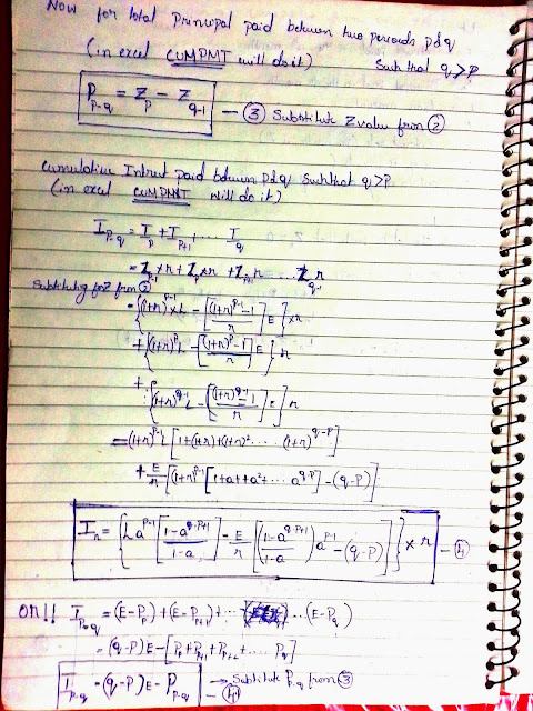
CUMIPMT and CUMPRINC  are two neat formulas that excel provides to calculate the cumulative Principal paid between two periods and cumulative  Interest paid between two periods respectively.

Now these formula are not available in all software we use. For example Tableau does not have it. So when I was writing the blog "Advantage; Homeloan" using the tool I had to derive the formulas myself. If you need to use them here are the formulas with derivation. (sorry did not have the patience to make re do this on the system)

                  

This is Appendix Just in case you need it

Using Fuzzy Lookup add-in in Excel.

Here is the problem.  I have the list of MPs (members of parliament) and their attendance register. I just wanted to see which party records better attendance and which states register better attendance.

But the problem is the mapping the names of these MPs from the two lists. One lists has the name Chowdhary,Smt. Santosh and the other list has Smt Santosh Chowdhary. (Notice the , and . after Smt)

These differences in Names will not allow me to map the names from two lists. 

Get the two lists in the same sheet. Make sure they are two different tables.

Click on go. Make sure the active cell is I an empty cell with enough space to populate the matched columns.

And boom! There it is…. Smt Santosh Chowdhary and Chowdhary,Smt. Santosh are matched. It also gives you percentage of similarity. So you can easily pick the wrong matches. (if there are)

Finding the Median in T-SQL

Median is a good measure of central tendency in many cases, especially when the distribution is skewed. This mode function is readily available in excel, but you will be surprised; T-SQL does not have a median function.

What is median?

Median is the middle value when sorted in order. If you have 7 values then the 3^rd value is the median. If there are even, say 10 elements in the set then it is average of 5^th and 6^th value.

Example: Let’s say our ages are as follows (note that they are sorted by age) median is 5

SL NO	Age
1	2
2	3
3	5
4	5
5	6
6	10
7	15

If we had another row then our median age would have been (5+6)/2

SL NO	Age
1	2
2	3
3	5
4	5
5	6
6	10
7	15
8	15

So if you have a hundred million rows you cannot do a quick

SELECT MEDIAN ([AGE])  FROM TABLE1

Nor can you paste the data on to excel and get the median because the data you have exceeds the number of rows excel can handle.

Here is the solution I am offering: (although this solution is not very novel it works well) sort the table by age (or the variable that you wish to find the mean for) and a row number for every row.  Then get the average of [(n+1)/2]+.25 and [(n+1)/2]-.25 th elements rounded off to the nearest whole number. ( where n is the total count of rows.) . This way if the count of row number is odd, let's say is 5 then we average 3^rd and 3^rd elements. If it is even say 6 then we average 3^rd  and 4^th elements.

 Example query: (Here, say, we are required to get the median age per country)

With CTE_AGE_RNK as(

select [SLNo]

,[Country]

      ,[Age]

,ROW_NUMBER() OVER(PARTITION by Country ORDER by  [AgeAtInterest])[rnk]

      ,cast (COUNT(1) over(PARTITION by I. Country ) AS decimal)[cnt] /*this is needed*/

from Table1 I (NOLOCK)

)

SELECT 

Country, avg([Age]) from CTE_AGE_RNK C

where  rnk IN (  ROUND(((([cnt]+1)/2)-0.25),0),ROUND(((([cnt]+1)/2)-0.25),0))

GROUP BY Country

Counting Distinct Values in Excel

Very recently some one had posted an excel problem on LinkedIn. The user wanted to get a count of distinct values. Microsoft offers a solution to this need.

={=SUM(IF(FREQUENCY(IF(LEN(A2:A10)>0,MATCH(A2:A10,A2:A10,0),""), IF(LEN(A2:A10)>0,MATCH(A2:A10,A2:A10,0),""))>0,1))}

http://office.microsoft.com/en-in/excel-help/count-occurrences-of-values-or-unique-values-in-a-data-range-HP003056118.aspx

 But the user wanted to count unique values from multiple columns, and the above formula cannot achieve that. (that is because the match function can handle only a single column/row array)

 A Much simpler and more effective formula is

 {=SUM(IFERROR(1/COUNTIF(A$2:A$10,A$2:A$10),""))}

 You could conveniently extend it to multiple rows.

 {=SUM(IFERROR(1/COUNTIF(A$2:C$10,A$2:C$10),""))}

What the formula does is, it counts the number of occurrences and find its reciprocal and add them all up. So, if "Apple" occurs 5 times in your array, the formula adds 1/5 5 times.

Distinct function is one of the most sought-after functions for spreadsheet users from across the world. Microsoft should introduce this function in their future updates. Remove duplicates , feature sometimes simply does not suffice.

Note:
the formulas with flower brackets are array formulas. You need to press CRTL+SHIFT+ENTER to get them to work.
Tip: Enter the formula without flower-brackets  The Cell will read #VALUE!. go back to the cell and hit F2 and then CRTL+SHIFT+ENTER